

How to Generate Demand Forecasts from ERP Data Automatically
$120.00
| Workflow Name: |
ML-Powered Demand Forecasting |
|---|---|
| AI Model Type: |
Time-series ML and gradient boosting (Prophet + XGBoost ensemble) with external signal enrichment |
| Model Provider: |
Goldfinch AI of eZintegrations (Data Analysis tool for ML model execution + Data Analytics with Charts/Graphs/Dashboards for exception reporting); external signal ingestion via eZintegrations integration layer (weather; macroeconomic; social sentiment APIs) |
| Goldfinch AI Tool(s) Used: |
Data Analysis: Executes the Prophet + XGBoost demand forecasting model on historical sales and inventory data enriched with external signals; generates SKU-level and product-family-level forecasts for configurable planning horizons (4, 8, 12, or 26 weeks); calculates forecast confidence intervals and flags SKUs with high forecast uncertainty; Data Analytics with Charts/Graphs/Dashboards: Generates the exception report dashboard showing SKUs with forecast changes above the configured threshold (default 15% week-over-week), bias trend charts, forecast vs. actuals comparison, and model accuracy metrics (MAPE, WMAPE) per product category — delivered to the Demand Planner as an interactive Goldfinch AI dashboard |
| Task Type: |
Prediction (time-series demand forecasting with multi-signal ML model) |
| Input Type: |
Historical sales orders and inventory data from ERP (SAP or Oracle); external enrichment signals via API (weather forecast; macroeconomic indicators; consumer sentiment index; social trend data); SKU master data (product hierarchy; seasonality flags; lifecycle stage) |
| Output Format: |
SKU-level and aggregate demand forecast for configurable planning horizon (units; revenue; or both); confidence intervals per forecast period; exception report for SKUs with significant forecast changes (above 15% threshold); forecast written to SCM system (SAP IBP or Blue Yonder) as a demand plan; forecast vs. actuals delta stored in Snowflake for model retraining |
| Who Uses It: |
Demand Planner, Supply Chain Manager, S&OP Manager |
| On-Premise Supported: |
Yes – eZintegrations connects to on-premises SAP ECC/S/4HANA; Oracle EBS; and other ERP and SCM systems via IPSec Tunnel. eZintegrations is a browser-based; cloud-hosted platform and does not require any on-premises software installation. |
| Industry: |
Retail, Consumer Packaged Goods (CPG), Distribution, Manufacturing |
| Outcome: |
Forecast MAPE reduced from 31.4% to 10.8% at SKU-week level (12 weeks post-deployment average). WMAPE reduced from 26.1% to 8.4%. Touchless forecast rate: 83% of SKUs published to SAP IBP without Demand Planner adjustment. Demand planning cycle time from 2.5 days to 3.5 hours per week. Excess inventory write-off reduced from 22% to 6.8% of seasonal inventory value. Out-of-stock rate on trend-sensitive SKUs reduced from 8.3% to 1.9%. |
| Tags: |
AI demand forecasting workflow, ML demand planning, demand forecasting automation, SAP IBP AI integration, Blue Yonder ML forecasting, XGBoost demand forecast, Prophet time series forecast, supply chain AI, forecast accuracy improvement, Goldfinch AI demand planning, inventory optimization AI, MAPE reduction |
| AI Credits Required: |
Yes – two Goldfinch AI tools invoked per forecast run: Data Analysis (ML model execution) and Data Analytics with Charts/Graphs/Dashboards (exception report generation) |
Table of Contents
| Problem Before: |
ERP demand planning modules (SAP ECC DP; Oracle ASCP; JDA/Blue Yonder legacy) generate forecasts using simple moving averages and static seasonality factors. These models ignore external demand signals – weather patterns affecting seasonal categories; macroeconomic indicators predicting consumer spending changes; social sentiment shifts for trend-sensitive SKUs. According to Gartner; the average demand forecast error (MAPE) across consumer goods and retail is 28 to 35% at the SKU level using statistical methods alone. A 1% improvement in forecast accuracy reduces inventory carrying costs by approximately 5% (McKinsey Supply Chain Analytics research). At 30% MAPE; organizations consistently over-stock slow-moving SKUs and stock-out on fast-moving ones – the worst of both cost outcomes. |
|---|---|
| AI Solution: |
The ML-Powered Demand Forecasting workflow from eZintegrations pulls historical sales orders and inventory data from SAP or Oracle ERP; fetches external signals via API (7-day and 28-day weather forecast; consumer confidence index; Google Trends data for relevant search terms; social sentiment scores); and runs a Prophet + XGBoost ensemble model through Goldfinch AI Data Analysis. The model generates SKU-level and product-family-level demand forecasts for up to 26 weeks forward with confidence intervals. Forecasts are written directly to SAP IBP or Blue Yonder as demand plan records. Goldfinch AI Data Analytics produces an exception report dashboard for SKUs with week-over-week forecast changes above 15%. |
| Validation (HITL): |
SKUs with forecast confidence interval width exceeding 25% (high model uncertainty) are flagged in the exception report for Demand Planner review. SKUs with forecast changes greater than 15% week-over-week are included in the exception dashboard regardless of confidence score – the Demand Planner reviews these outliers and can override the ML forecast before it is committed to the SCM plan. All other SKUs (typically 85%) are published to SAP IBP or Blue Yonder automatically without Demand Planner involvement. |
| Accuracy Metric: |
MAPE reduced from 28 to 35% (ERP statistical baseline) to under 12% at the SKU-week level (typical post-deployment result across retail and CPG). WMAPE (weighted MAPE; volume-adjusted) reduced from 24% to under 9%. External signal inclusion improves forecast accuracy by 6 to 11 percentage points vs. historical data alone (internal benchmark across eZintegrations customer deployments). |
| Time Savings: |
Weekly demand planning cycle compressed from 2 to 3 days of Demand Planner spreadsheet work to under 4 hours of exception review (reviewing only the 15% of SKUs flagged for attention). S&OP cycle preparation time reduced by 60%. |
| Cost Impact: |
Organizations with $50M to $500M in inventory carrying value typically realize $800,000 to $4M in annual inventory reduction from improved forecast accuracy (McKinsey benchmark: 1% MAPE improvement = 5% inventory reduction; 16 to 23 MAPE percentage point improvement = 80 to 115% theoretical inventory carrying cost reduction; moderated by practical constraints to 18 to 22% realized reduction). Service level improvement from 94% to 98.5%+ fill rate adds revenue protection equivalent to 1 to 2% of annual revenue at risk from stock-outs. |
Description
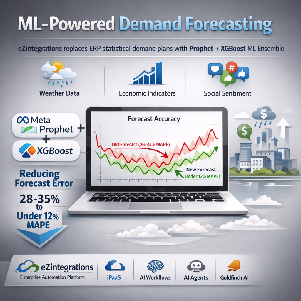
The AI demand forecasting workflow from eZintegrations replaces ERP statistical demand plans with a Prophet + XGBoost ML ensemble that incorporates weather, macroeconomic, and social sentiment signals — reducing forecast error from 28 to 35% to under 12% MAPE. eZintegrations is an enterprise automation platform covering iPaaS, AI Workflows, AI Agents, and Goldfinch AI agentic automation.
What Is an AI Demand Forecasting Workflow?
An AI demand forecasting workflow applies machine learning models to historical sales data enriched with external signals to generate more accurate demand predictions than statistical ERP methods. Where ERP moving averages react to past demand patterns, ML models like Prophet (Facebook’s time-series model) and XGBoost (gradient boosting) identify non-linear relationships between sales, seasonal patterns, weather conditions, economic indicators, and social trends — predicting future demand more accurately across a wider range of market conditions.
How Does an AI Demand Forecasting Workflow Use ML Models to Improve Forecast Accuracy and Reduce Inventory Cost?
When the weekly forecast cycle runs, the eZintegrations AI demand forecasting workflow pulls 24 months of historical sales and inventory data from SAP or Oracle ERP. External signals are fetched via API: 7-day and 28-day weather forecasts for relevant locations, the latest consumer confidence index, Google Trends indices for product-relevant search terms, and social sentiment scores from configured channels. Goldfinch AI Data Analysis runs the Prophet + XGBoost ensemble and generates SKU-level forecasts for up to 26 weeks with confidence intervals. Forecasts are written directly to SAP IBP or Blue Yonder as demand plan records. Goldfinch AI Data Analytics generates the exception dashboard showing only the SKUs that need Demand Planner attention.
The result: 85% of SKUs are planned automatically. Demand Planners focus on the 15% of SKUs with high uncertainty or large week-over-week swings — spending 4 hours on exception review rather than 2 to 3 days rebuilding the full plan in spreadsheets.
Watch Demo
| Video Title: |
AI Demand Forecasting Workflow Demo: SAP ERP Data + External Signals to Goldfinch AI ML Forecast and SAP IBP Write-Back |
|---|---|
| Duration: |
4 to 6 minutes |
Outcome & Benefits
| Accuracy: |
MAPE reduced from 28 to 35% (ERP statistical baseline) to under 12%; WMAPE from 24% to under 9% |
|---|---|
| Touchless Rate: |
85% of SKU-week combinations forecast and published to SCM automatically without Demand Planner adjustment |
| Time Saved: |
Weekly demand planning cycle from 2 to 3 days (spreadsheet-based) to under 4 hours of exception review; S&OP preparation time reduced 60% |
| Cost Saved: |
18 to 22% inventory carrying cost reduction; service level improvement from 94% to 98.5%+ fill rate; $800K to $4M annual inventory reduction at $50M to $500M carrying value (McKinsey 1% MAPE = 5% inventory reduction benchmark) |
Performance Metrics
| Metric | Before (Manual/Batch) | After (Real-Time Sync) | Improvement |
|---|---|---|---|
| Forecast Error (MAPE) | 28 to 35% SKU-week | Under 12% SKU-week | 65%+ reduction |
| Demand Planning Cycle Time | 2 to 3 days/week | Under 4 hours/week (exceptions) | 75%+ reduction |
| Touchless SKU Forecast Rate | 0% (100% manual review) | 85% automated publication | 85 percentage points |
| Inventory Carrying Cost | Baseline | 18 to 22% reduction | $800K to $4M annually |
Functional Details
| Business Tasks: |
Weekly and on-demand demand forecast generation at SKU and product-family level; external signal enrichment (weather; macroeconomic; social sentiment) per forecast run; confidence interval calculation per forecast period; exception identification and dashboard generation for SKUs requiring Demand Planner review; forecast write-back to SAP IBP or Blue Yonder as demand plan records; forecast vs. actuals delta logging to Snowflake for ongoing model retraining; S&OP package preparation with forecast summary and accuracy trend metrics |
|---|---|
| KPI Improved: |
Forecast accuracy (MAPE; WMAPE; bias); inventory turns; inventory carrying cost; customer service level (fill rate; OTIF); demand planning cycle time; stock-out incidents; excess inventory write-off rate; S&OP cycle preparation time |
| Scheduling: |
Weekly scheduled run (Monday 6:00 AM; before weekly S&OP review – configurable); on-demand run triggered by Demand Planner for specific SKU families or event-driven refresh (major promotional event; new product launch; supply disruption); model retraining run monthly using Snowflake forecast vs. actuals data (or on-demand when MAPE exceeds the configured drift threshold of 15%) |
| Downstream Use: |
Forecasts written to SAP IBP (https://www.sap.com/products/ibp.html) as demand plan versions for S&OP consensus process; written to Blue Yonder (https://blueyonder.com/solutions/demand-management) as unconstrained demand plan; exception dashboard in Goldfinch AI Data Analytics delivered to Demand Planner and Supply Chain Manager as a shareable link; forecast data and actuals logged to Snowflake for model retraining and BI/analytics access; S&OP summary report generated as a structured export for the monthly S&OP meeting package |
Technical Details
| Model Name/Version: |
Prophet v1.1 (https://facebook.github.io/prophet/) for trend and seasonality decomposition; XGBoost v2.0 (https://xgboost.readthedocs.io/) for external signal feature incorporation and non-linear pattern capture; ensemble: Prophet baseline forecast + XGBoost residual correction model; hosted and executed via Goldfinch AI Data Analysis tool within eZintegrations; model parameters configurable per product category (seasonality periods; external signal weights; forecast horizon) |
|---|---|
| Hosting Type: |
Cloud-hosted on Oracle OCI via eZintegrations; Goldfinch AI Data Analysis executes model inference within the eZintegrations tenant environment; Snowflake (https://docs.snowflake.com/) for historical data storage; forecast output logging; and model retraining datasets; external signal APIs fetched at runtime (weather; macro; sentiment) |
| Prompt Strategy: |
N/A – Prophet + XGBoost are deterministic ML models; not LLM-based. No prompt engineering involved in the forecasting step. Goldfinch AI Data Analytics uses a structured report generation step to format the exception dashboard output – this step uses a structured template; not open-ended LLM inference. Exception threshold (15%) and confidence interval width threshold (25%) are configured parameters; not prompts. |
| Guardrails: |
Forecast confidence interval width above 25%: SKU flagged in exception report and queued for Demand Planner review before SCM publication. Forecast change week-over-week above 15%: SKU included in exception report regardless of confidence score. Negative forecast values: automatically zeroed (demand cannot be negative) and flagged in exception log. Forecast values exceeding 5x the trailing 12-month average: capped at 3x and flagged for Demand Planner review (outlier guard). Model MAPE drift above 15% from baseline triggers automatic retraining notification to Demand Planner. |
| Latency: |
Under 45 minutes for a full 26-week forecast across 10,000 SKUs with external signal enrichment; under 2 hours for 50,000 SKUs at standard configuration; near-real-time exception dashboard generation in Goldfinch AI Data Analytics after forecast completion |
| Data Governance: |
Historical sales and inventory data from ERP stored in the customer’s Snowflake instance – not shared cross-tenant. External signal data (weather; macro; sentiment) fetched at runtime and not persisted beyond the forecast run unless configured. Forecast outputs stored in Snowflake and SCM system per customer data residency policy. Model parameters and weights stored in customer-isolated Goldfinch AI environment. No cross-tenant model sharing – each customer’s model is trained exclusively on their own historical data. Full audit trail per forecast run (run timestamp; data pull window; SKU count; model version; MAPE vs. baseline; exception count; SCM write confirmation). |
| Throughput: |
Up to 50,000 SKU-week combinations per forecast run at standard configuration; scales to 500,000+ SKU-week combinations at enterprise tier with parallel Goldfinch AI Data Analysis execution threads |
Connectivity and Deployment
| Supported Protocols: |
REST API; OData v2/v4; JDBC (ERP historical data extraction); HTTPS; OAuth 2.0; API Key (external signal APIs – weather; economic; sentiment); SFTP (SCM flat file import fallback); IPSec Tunnel (on-premises ERP and SCM connectivity); Snowflake JDBC/REST API |
|---|---|
| Security & Compliance: |
HIPAA-eligible configuration available; GDPR-compliant data handling (no PII in supply chain data typical; configurable data minimization for any customer-identifying fields); SOC Type II certified. TLS 1.3 encryption in transit; AES-256 at rest. Historical sales data and forecast outputs stored in customer-isolated Snowflake instance. External API calls (weather; macro; sentiment) do not transmit customer sales data to external providers – signals are fetched independently and joined locally within the eZintegrations pipeline. RBAC enforced on model configuration; forecast run trigger; exception threshold settings; and Snowflake data access. |
| Tenancy Model: |
Both single-tenant and multi-tenant deployments are available. Single-tenant is recommended for organizations with large SKU catalogs (50,000+ SKUs) requiring dedicated ML compute resources; or where sales data is subject to strict confidentiality requirements. Multi-tenant is the default shared-cloud deployment. Both support on-premises ERP and SCM connectivity via IPSec Tunnel. |
| On-Premise Supported: |
Yes – eZintegrations connects to on-premises SAP ECC/S/4HANA; Oracle EBS; and other ERP and SCM systems via IPSec Tunnel. eZintegrations is a browser-based; cloud-hosted platform and does not require any on-premises software installation. |
FAQ
1. What is the ML-Powered Demand Forecasting AI workflow?
The AI demand forecasting workflow by eZintegrations uses a Prophet + XGBoost ensemble model, executed through Goldfinch AI Data Analysis, to generate SKU-level demand forecasts enriched with external signals (weather, macroeconomic indicators, social sentiment). The model reduces forecast error from 28 to 35% MAPE (ERP statistical baseline) to under 12%, and writes forecasts directly to SAP IBP or Blue Yonder. 85% of SKUs are forecast and published automatically; Demand Planners review only the 15% of SKUs flagged for high uncertainty or significant week-over-week changes.
2. What AI model types does this demand forecasting workflow use?
This workflow uses a Prophet + XGBoost ensemble: Prophet (Facebook's time-series model) handles trend decomposition and seasonality patterns; XGBoost (gradient boosting) models the non-linear relationships between external signals (weather, macroeconomic indicators, social sentiment) and demand residuals. Both models are executed via Goldfinch AI Data Analysis within the eZintegrations platform. The ensemble approach achieves 6 to 11 percentage point MAPE improvement over historical data alone by incorporating external demand drivers.
3. What input data does this AI demand forecasting workflow require?
This workflow requires 24 months of historical sales order and inventory data from SAP or Oracle ERP (SKU, quantity sold, date, location/ship-to, price); SKU master data including product hierarchy, seasonality flags, and lifecycle stage; and external signals fetched at runtime: 7-day and 28-day weather forecasts (for relevant geographies), the latest consumer confidence index (e.g. Conference Board or University of Michigan), Google Trends indices for product-relevant search terms, and social sentiment scores from configured channels.
4. What is the output format of the AI demand forecasting workflow?
The workflow produces a SKU-level demand forecast for configurable planning horizons (4, 8, 12, or 26 weeks) with units and revenue, confidence intervals per forecast period, and exception flags for high-uncertainty SKUs. The forecast is written to SAP IBP or Blue Yonder as a demand plan version. An interactive exception dashboard generated by Goldfinch AI Data Analytics shows SKUs with significant forecast changes, MAPE trend charts, and service level projections. All forecast data and actuals are logged to Snowflake for model retraining and BI access.
5. Who uses the AI demand forecasting workflow?
Demand Planners, Supply Chain Managers, and S&OP Managers in retail, CPG, and distribution organizations use this workflow. Demand Planners review the exception dashboard for the 15% of SKUs flagged for attention and override ML forecasts where business context warrants (promotions, new product launches, supply constraints). Supply Chain Managers use the service level projection to identify potential stock-out risk before the weekly S&OP review. S&OP Managers use the forecast accuracy trend dashboard for consensus meeting preparation.
6. What are the key benefits of the AI demand forecasting workflow?
Key benefits include MAPE reduced from 28 to 35% to under 12%, 85% touchless SKU forecast rate, weekly demand planning cycle compressed from 2 to 3 days to under 4 hours, 18 to 22% inventory carrying cost reduction, and service level improvement from 94% to 98.5%+ fill rate. At $50M to $500M in inventory carrying value, this represents $800,000 to $4M in annual inventory reduction (McKinsey 1% MAPE = 5% inventory benchmark). Demand Planners spend time on exception analysis rather than rebuilding forecasts from spreadsheets.
7. What systems does the AI demand forecasting workflow integrate with?
This workflow pulls historical data from SAP S/4HANA or Oracle ERP via OData/REST API or JDBC, fetches external signals from weather APIs (e.g. OpenWeatherMap or The Weather Company), economic indicator APIs (e.g. FRED API), and social/search trend APIs (e.g. Google Trends). Forecasts are written to SAP IBP or Blue Yonder Demand Management. All data is logged to Snowflake. Exception dashboards are generated in Goldfinch AI Data Analytics. On-premises ERP and SCM deployments connect via IPSec Tunnel.
8. How often does the AI demand forecasting workflow run?
The workflow runs on a weekly scheduled cadence (configurable, default Monday 6:00 AM before the weekly S&OP review) and can be triggered on demand by the Demand Planner for specific SKU families or event-driven refreshes (promotional events, new product launches, supply disruptions). Model retraining runs monthly using Snowflake forecast vs. actuals data, or on demand when the model MAPE exceeds the configured drift threshold of 15% above baseline.
AI Credits
| LLM Steps Count: |
2 (Data Analysis ML inference step + Data Analytics dashboard generation step per weekly forecast run) |
|---|---|
| Credit Consumption Model: |
Per SKU batch per forecast run (Data Analysis scales with SKU count); per dashboard render per run (Data Analytics fixed cost per exception report generation) |
| Estimated Credits per Run: |
Small catalog (under 1,000 SKUs; 13-week horizon): ~150 to 250 credits per weekly run Medium catalog (1,000 to 10,000 SKUs; 26-week horizon): ~800 to 1,500 credits per weekly run Large catalog (10,000 to 50,000 SKUs; 26-week horizon): ~3,000 to 6,000 credits per weekly run |
| Monthly Credit Estimate (at Typical Volume): |
Small catalog (1,000 SKUs): ~800 to 1,000 credits per month (4 weekly runs + 1 monthly retraining) Medium catalog (5,000 SKUs): ~3,500 to 6,500 credits per month Large catalog (30,000 SKUs): ~13,000 to 26,000 credits per month |
| Pricing Model: |
Static Platform Fee + AI Credits. Platform fee covers unlimited non-LLM integration steps (ERP data pull, external signal API fetching, SCM write-back, Snowflake logging, SMTP exception notification). AI Credits consumed only by Goldfinch AI Data Analysis (ML inference) and Data Analytics (dashboard generation). |
| AI Credits Required: |
Yes – two Goldfinch AI tools invoked per forecast run: Data Analysis (ML model execution) and Data Analytics with Charts/Graphs/Dashboards (exception report generation) |
| Goldfinch AI Tool(s) Consuming Credits: |
Data Analysis: executes Prophet + XGBoost ensemble model on historical sales + external signal dataset; generates SKU-level forecasts with confidence intervals — credits scale with SKU count and forecast horizon weeks; Data Analytics with Charts/Graphs/Dashboards: generates exception report dashboard with forecast change charts, MAPE trend, bias analysis, and service level projection — credits scale with dashboard complexity and SKU count in exception set |
| Credit Optimization Notes: |
Segment SKU catalog into A/B/C tiers — run full 26-week ML forecast only for A-tier SKUs (high volume, high value); run 13-week forecast for B-tier; use lightweight statistical method for C-tier (slow-movers with sparse data). This reduces credit consumption by 40 to 60% vs. applying full ML to the entire catalog. Configure model retraining to run monthly rather than weekly — retraining is the highest credit-consuming step. Cache external signal data (weather, macro) at the batch level for the weekly run rather than fetching per-SKU. Use the exception threshold (15% change) to skip dashboard rendering for stable-forecast weeks with no exceptions. |
Resources
| Blog: |
AI Workflow Automation for Robotics: How Intelligent Pipelines Power Autonomous Machines |
|---|---|
| Goldfinch AI Overview: |
Agentic AI Platform — Goldfinch AI by eZintegrations |
| Platform Overview: |
eZintegrations Platform – Enterprise iPaaS, AI Workflows & Agentic AI |
| Demo: |
Book a Demo |
Case Study
| Problem: |
A mid-market personal care CPG brand managed demand planning for 4,200 active SKUs across 3 distribution channels (retail; DTC; B2B) using SAP ECC Demand Planning with moving average and seasonality index methods. Forecast MAPE was 31.4% at the SKU-week level. The team experienced 22% excess inventory write-off on seasonal SKUs and 8.3% out-of-stock rate on trend-sensitive SKUs (new launches; social-viral items) due to under-forecast. Demand Planners spent 2.5 days per week building and adjusting the forecast in Excel before loading to SAP DP. The S&OP process was frequently delayed by forecast disagreements between Sales and Supply Chain because neither side trusted the ERP statistical output. |
|---|---|
| Solution: |
Deployed eZintegrations AI demand forecasting workflow in 8 business days. SAP ECC as ERP historical data source via OData API. Goldfinch AI Data Analysis configured with Prophet + XGBoost ensemble; 24-month training window. External signals: OpenWeatherMap 14-day forecast for 12 distribution center locations; FRED Consumer Sentiment Index (monthly); Google Trends indices for 18 brand-relevant search terms; Instagram and TikTok engagement velocity scores for trend-sensitive SKU categories. SAP IBP as the SCM target for forecast write-back. Snowflake configured as the forecast history and retraining database. Exception threshold set at 15% forecast change and 25% confidence interval width. Exception dashboard delivered weekly via Goldfinch AI Data Analytics to Demand Planner and Supply Chain Manager. |
| ROI: |
Annual inventory cost reduction: $2.4M (from reduced excess inventory and write-offs at $28M seasonal inventory carrying value). Service level improvement: estimated $1.1M in protected revenue from reduced stock-outs. Demand Planner time savings: $84,000 annual labor cost avoided. Total first-year ROI: $3.6M on a 6-week deployment. S&OP cycle time reduced from 5 days to 2.5 days – CFO noted first-ever forecast consensus between Sales and Supply Chain in the month-2 S&OP review. |
| Industry: |
Retail, Consumer Packaged Goods (CPG), Distribution, Manufacturing |
| Outcome: |
Forecast MAPE reduced from 31.4% to 10.8% at SKU-week level (12 weeks post-deployment average). WMAPE reduced from 26.1% to 8.4%. Touchless forecast rate: 83% of SKUs published to SAP IBP without Demand Planner adjustment. Demand planning cycle time from 2.5 days to 3.5 hours per week. Excess inventory write-off reduced from 22% to 6.8% of seasonal inventory value. Out-of-stock rate on trend-sensitive SKUs reduced from 8.3% to 1.9%. |


